Clustering the Stars

Hertzsprung–Russell diagram for about 1000 nearest stars from Gliese catalogue
You may create such diagram uploading our data file to MS-Excel.

Popular task in data processing is about clustering the samples - i.e. splitting the whole set of data points into the groups of related or close ones. There exist different approaches to clustering and we'll now try one of the most popular - based on density of points - it is called DBSCAN. Besides data processing it could be very handy in finding regions in images for example.

Let us take the Gliese Catalogue of Nearest Stars, its 2-nd edition. For every star we'll take only:

• its catalogue index (like GLxxx.x where x-s are some digits);
• color as a B-W Color Index - value roughly between -0.3 and 1.4, going through blue, white, yellow, red stars;
• absolute magnitude - how bright the star would be seen from distance about 33 light years (roughly from 0 to 10 - the more, the dimmer).

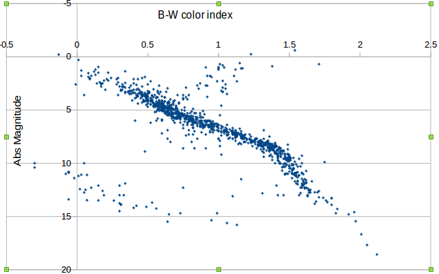
If we try to plot this data on a chart, we'll get famous picture, similar to one shown above - Hertzsprung-Russell diagram. It shows that stars of given color usually tend to have some specific magnitude (and therefore some specific size) - i.e. there is a strong correlation.

However it also shows that there is more than one "line" of this correlation. Most of stars fall into the line called Main Sequence, but there are also a group of hot but small stars (in the lower left corner) - they are White Dwarfs. Really there could be more separate groups found, but for now it is not that important.

DBSCAN algorithm description

To find such groups not with our eyes, but with the help of computer, we can apply clustering to these data. Let us try the approach which is explained below.

1. We regard any data sample as a point in space (in our case it is just 2D space since we have only two axes - color and magnitude).
2. Choose two values eps and minPoints. The cluster could not have less than minPoints points while eps is a kind of maximum distance between neighbor points in the cluster.
3. Let us call the core-point any which have at least minPoints - 1 neighbors at distance not exceeding eps.
4. To create the core of the cluster, find any core-point then proceed adding any other core-points which lay not further than eps from any of points already included in the core of the cluster. It is like growing the snowball.
5. When no more core-points could be found to add to the cluster - we should add any other non-core points found within eps distance from the points of the cluster's core.
6. Now proceed with searching for next clusters, repeat from 3 until no more unvisited core-points found.
7. All remaining points are considered as noise.

The very important step yet omitted is to normalize axes before step 2. Why is it necessary? You see that even for our example, the range of colors (-0.3 ... 1.4) is roughly 5 times less than the range of magnitudes (0 ... 10) so the distances by one axis are incomparable with distances by another. This surely will spoil calculation of distance between points by Pythagorean formula. Normalization will scale and shift axes to roughly similar values. Here is the simple algorithm:

• for chosen axis (e.g. color or magnitude values) calculate their average (i.e. sum and divide by amount);
• then calculate their corrected standard deviation which have sense of average distance from the average value: s = sqrt( sum( (Xi - avg)^2 ) / (n-1) ) - here Xi are values and n is their amount;
• at last each value should be scaled and shifted as Xi' = (Xi - avg) / s - that's all.

For example if we have color values of 4 stars like 10, -20, 5, -5 then after such normalization they become 0.945 -1.323 0.567 -0.189.

Problem Statement

Download data-file here (CSV-format)

The data are in CSV format, the first line is a header and should be skipped. You will be told how many data samples to take from the beginning of this list (e.g. first 500 lines), and what values of minPoints and eps to use. You need to return sizes of clusters you get in decreasing order.

Input data: will contain N (amount of lines to take) followed by minPoints and eps.
Output: should contain several integers - sizes of clusters in decreasing order.

Example:

input data:
700 3 0.375000

output data:
666 10 6 5 3

Another Example:

input data:
900 3 0.250000

output data:
818 17 13 8 6 4 3